A jam can travel backward.
Cars move right, but holes move left through a crowded region. In the space-time plot, follow the empty cells: a pattern can travel against the motion of its parts.
THE NEXT QUESTION IS YOURS
A rule is only half the story. The starting state, the edges, and the time you observe can change what you see.
Make a comparison. Test an intuition. Take the evidence with you.
Start with a guided investigationAll measurements come from the complete run. The generation inspector lets you look at one row at a time.
Rule 90, identical beginnings, different edges. Look beyond generation 64, when the growing pattern can reach a boundary.
Opening the laboratory…
GENERATION INSPECTOR
Scrub to inspect both worlds. Time runs down each diagram; scroll inside a plot to explore its full history.
A SMALL CHANGE, MEASURED
Within each experiment, toggle the central starting cell, rerun the same rule, and count the cells that disagree. This compares each run with its own perturbation.
Every generation, including the initial state. Values are percentages of the world width.
| Generation | A difference (%) | B difference (%) |
|---|
TAKE THE EVIDENCE
The session includes both rules, starting rows, boundaries, exact trajectories, measurements, and the traffic run. PNG exports contain the selected view at integer pixel scaling.
CSV includes density, activity, and perturbation difference for every generation.
A REAL QUESTION. AN IDEALIZED MODEL.
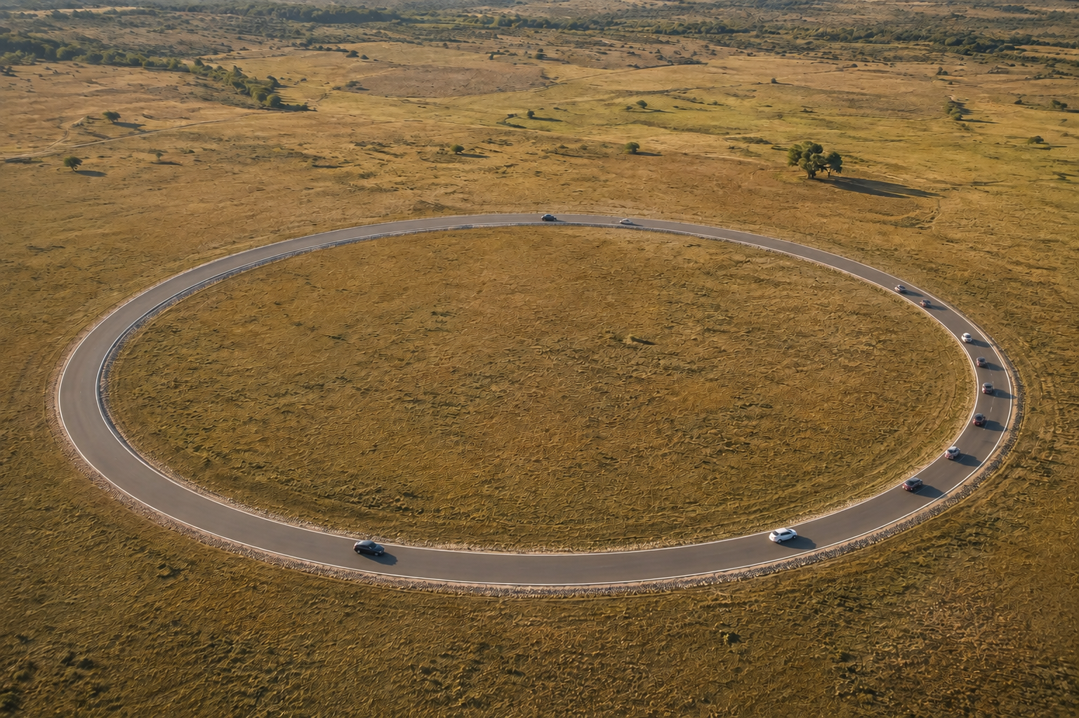
On this 128-cell ring, a car advances one cell to the right if that cell is empty. All cars update together. Add cars and observe when empty space becomes the limiting resource.
Density: 0.500 cars per cell
An exact car count, placed with a deterministic shuffle. Rearranging changes the transient, while the car count stays fixed.
Flow is car moves per road cell per update. A moving car’s speed is one cell per update. These are dimensionless model quantities, with no conversion to vehicles per hour.
Ring snapshot · generation Movement →
TEST THE ENTIRE RANGE
One computed run for every possible car count. Solid line: observed flow over updates 129–256. Dashed line: the long-run Rule 184 reference, q = min(ρ, 1 − ρ).
Calculating all 129 car counts…
| Cars | Density | Observed flow | Reference flow |
|---|
Cars move right, but holes move left through a crowded region. In the space-time plot, follow the empty cells: a pattern can travel against the motion of its parts.
At low density, cars limit the flow. Above half occupancy, empty cells limit it. A full ring has no space to move, so its flow is zero.
Every car is identical. There is no braking delay, lane change, reaction time, road entry, or randomness during an update. This model isolates exclusion; it is not a calibrated traffic predictor.
Click a cell to toggle it. For keyboard editing, enter the indices of every live cell below, separated by commas. An empty field means an empty world.
THE EIGHT NEIGHBORHOODS
Density and difference average all rows; activity averages transitions. Entropy measures live/dead balance, not complexity. These metrics always describe the primary run and its perturbation.